Vous êtes ici

Solution des exercices : Dynamique - Ts

Classe:

Terminale

Exercice 1

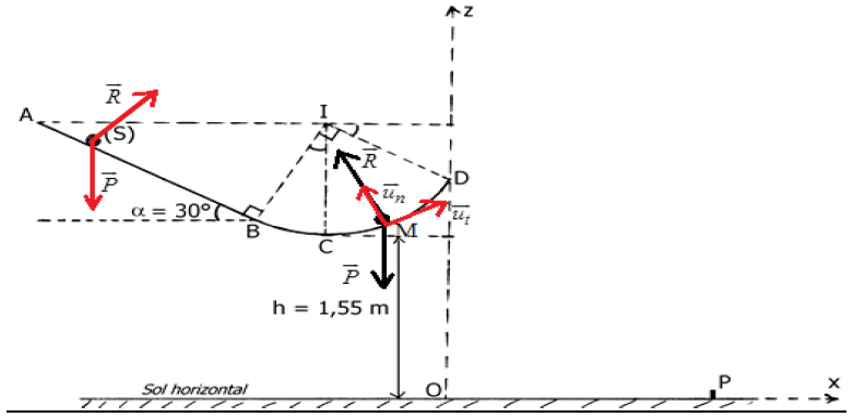
1) a) Vitesse du solide

$(S)$ en

$B$ , en

$C$ et en

$D$

$-\$ Système étudié : le solide

$(S)$

$-\$ Référentiel d'étude : terrestre supposé galiléen

$-\$ Bilan des forces appliquées : le poids

$\vec{P}$ et la réaction

$\vec{R}$ du plan

Le théorème de l'énergie cinétique s'écrit entre :

$\bullet\$ les points

$A\$ et

$\ B\ :$

$\begin{array}{rcl} \Delta\,E_{C}=\sum\overrightarrow{W}&\Rightarrow&\,E_{C_{B}}-E_{C_{A}}=W_{AB}(\vec{P})+W_{AB}(\vec{R})\\\\&\Rightarrow&\dfrac{1}{2}mv_{B}^{2}-0=mgAB\sin\alpha+0\\\\&\Rightarrow&v_{B}=\sqrt{2ABg\sin\alpha}\\\\&\Rightarrow&v_{B}=\sqrt{2\times 1.6\times 10\sin 30}\\\\&\Rightarrow&v_{B}=4.0\;m\cdot s^{-1} \end{array}$

$\begin{array}{rcl}\Delta\,E_{C}=\sum\overrightarrow{W}&\Rightarrow&E_{C_{C}}-E_{C_{B}}=W_{BC}(\vec{P})+W_{BC}(\vec{R})\\\\&\Rightarrow&\dfrac{1}{2}mv_{C}^{2}-\dfrac{1}{2}mv_{B}^{2}=mgr(1-\cos\alpha)+0\\\\&\Rightarrow&v_{C}=\sqrt{2gr(1-\cos\alpha)+v_{B}^{2}}\\\\&\Rightarrow&v_{C}=\sqrt{2\times 10\times 0.9(1-\cos 30)+4^{2}}\\\\&\Rightarrow&v_{C}=4.3\;m\cdot s^{-1} \end{array}$

$\bullet\$ les points

$C\$ et

$\ D\ :$

$\begin{array}{rcl}\Delta\,E_{C}=\sum\overrightarrow{W}&\Rightarrow&E_{C_{D}}-E_{C_{C}}=W_{CD}(\vec{P})+W_{CD}(\vec{R})\\\\&\Rightarrow&\dfrac{1}{2}mv_{D}^{2}-\dfrac{1}{2}mv_{C}^{2}=mgr(1-\cos\beta)+0\\\\&\Rightarrow&v_{D}=\sqrt{v_{C}^{2}-2gr(1-\cos\beta)}\\\\&\Rightarrow&v_{D}=\sqrt{(4.3)^{2}-2\times 10\times 0.9(1-\cos 60)}\\\\&\Rightarrow&v_{D}=3.0\;m\cdot s^{-1} \end{array}$

b) Intensité de la force

$\vec{R}$ exercée par la piste sur le solide

$(S)$ en

$C$ et en

$D$

$-\$ Système étudié : le solide

$-\$ Référentiel : terrestre supposé galiléen

$-\$ Bilan des forces appliquées : le poids

$\vec{P}$ du solide ; la réaction de la piste

$\vec{R}$

$-\$ Le théorème du centre d'inertie s'écrit :

$\vec{P}+\vec{R}=m\vec{a}$

Dans le repère de Frenet

$\left(M\;,\ \vec{u}_{t}\;,\ \vec{u}_{n}\right)$

$\vec{u}_{n}\ :$

$\begin{array}{rcl} -P+R=ma_{n}&\Rightarrow&-mg+R_{C}=m\dfrac{V_{C}^{2}}{r}\\\\&\Rightarrow&R_{C}=m\left(g+\dfrac{V_{C}^{2}}{r}\right)\\\\&\Rightarrow&R_{C}=50\cdot 10^{-3}\left(10+\dfrac{4.3^{2}}{0.9}\right)\\\\&\Rightarrow&R_{C}=1.5\end{array}$

$\begin{array}{rcl} -P\cos\theta+R=ma_{n}&\Rightarrow&-mg\cos\theta+R_{D}=m\dfrac{V_{D}^{2}}{r}\\\\&\Rightarrow&R_{D}=m\left(g\cos\theta+\dfrac{V_{D}^{2}}{r}\right)\\\\&\Rightarrow&R_{D}=50\cdot 10^{-3}\left(10\cos 60+\dfrac{3.0^{2}}{0.9}\right)\\\\&\Rightarrow&R_{D}=0.75\;N \end{array}$

c) Caractéristiques du vecteur vitesse

$\vec{V}_{D}$ du solide

$(S)$ au point

$D$

$-\$ Point d'application : le point

$D$

$-\$ Direction : tangente à la trajectoire au point

$D$

$-\$ Sens : dirigé vers le haut

$-\$ Intensité :

$v_{D}=3.0\;m\cdot s^{-1}$

2) a) Équation cartésienne de la trajectoire du mouvement de

$(S)$

Le solide est soumis à son poids

$\vec{P}$ ; dans le référentiel terrestre supposé galiléen, le théorème du centre d'inertie appliqué au solide

$(S)$ s'écrit :

$\begin{array}{rcl} \vec{P}=m\vec{a}&\Rightarrow&m\vec{g}=m\vec{a}\\\\&\Rightarrow&\vec{a}=\vec{g}\\\\&\Rightarrow&\vec{a}\left\lbrace\begin{array}{rcl}a_{x}&=&0\\a_{x}&=&-g \end{array}\right.\end{array}$

$\dfrac{\mathrm{d}\vec{V}}{\mathrm{d}t}=\vec{a}\ \Rightarrow\ \left\lbrace\begin{array}{rcl}V_{x}&=&cte\\V_{x}&=&-gt+cte \end{array}\right.$

Or,

$\ \left\lbrace\begin{array}{lllll}V_{x}(0)&=&cte&=&V_{D}\cos\theta\\\\V_{x}(0)&=&-g\times 0+cte&=&V_{D}\sin\theta \end{array}\right.$

Donc,

$\overrightarrow{V}\left\lbrace\begin{array}{lcl}V_{x}&=&V_{D}\cos\theta\\\\V_{x}&=&-gt+V_{D}\sin\theta \end{array}\right.$

Par suite,

$\begin{array}{rcl}\dfrac{\mathrm{d}\overrightarrow{OM}}{\mathrm{d}t}=\vec{V}&\Rightarrow&\overrightarrow{OM}\left\lbrace\begin{array}{rcl}x&=&(V_{D}\cos\theta)t+cte\\\\z&=&-\dfrac{1}{2}gt^{2}+(V_{D}\sin\theta)t+cte\end{array}\right.\\\\&\Rightarrow&\left\lbrace\begin{array}{lllll}x(0)&=&(V_{D}\cos\theta)\times 0+cte&=&0\\\\z(0)&=&-\dfrac{1}{2}g\times 0^{2}+(V_{D}\sin\theta)\times 0+cte&=&h+r(1-\cos\theta) \end{array}\right.\\\\&\Rightarrow&\left\lbrace\begin{array}{rclr}x&=&(V_{D}\cos\theta)t&(1)\\\\z&=&-\dfrac{1}{2}gt^{2}+(V_{D}\sin\theta)t+h+r(1-\cos\theta)&(2)\end{array}\right.\end{array}$

$(1)\ \Rightarrow\ x=(V_{D}\cos\theta)t\ \Rightarrow\ t=\dfrac{x}{V_{D}\cos\theta}$

$(1)$ dans

$(2)$ entraine :

$z=-\dfrac{1}{2}g\left(\dfrac{x}{V_{D}\cos\theta}\right)^{2}+(V_{D}\sin\theta)\left(\dfrac{x}{V_{D}\cos\theta}\right)+h+r(1-\cos\theta)$

$\boxed{\Rightarrow\;z=-\dfrac{1}{2}g\dfrac{x^{2}}{V_{D}^{2}\cos^{2}\theta}+x\tan\theta+h+r(1-\cos\theta)}$

b) Hauteur

$H$ au-dessus du sol horizontal

$\dfrac{\mathrm{d}z}{\mathrm{d}x}=-g\dfrac{x}{V_{D}^{2}\cos^{2}\theta}+\tan\theta=0\ \Rightarrow\ x=\dfrac{V_{D}^{2}\cos^{2}\theta}{g}\tan\theta$

Donc,

$\begin{array}{rcl} z&=&-\dfrac{1}{2}g\dfrac{\left(\dfrac{V_{D}^{2}\cos^{2}\theta}{g}\tan\theta\right)^{2}}{V_{D}^{2}\cos^{2}\theta}+\dfrac{V_{D}^{2}\cos^{2}\theta}{g}\tan\theta\tanh\theta+h+r(1-\cos\theta)\\\\&=&\dfrac{1}{2}\dfrac{V_{D}^{2}\cos^{2}\theta}{g}\tan^{2}\theta+h+r(1-\cos\theta)\\\\&=&\dfrac{1}{2}\dfrac{V_{D}^{2}\cos^{2}\theta}{g}+h+r(1-\cos\theta)\\\\&=&\dfrac{1}{2}\dfrac{3.0^{2}\sin^{2}60}{10}+1.55+0.9(1-\cos 60)\\\\&=&H=2\,m\end{array}$

c) Calcul de la distance OP où P est le point d'impact du solide

$(S)$ sur le sol horizontal

$\begin{array}{rcl} z_{1}&=&\dfrac{-\tan\theta+\sqrt{\tan\theta^{2}+2g\left(\dfrac{h+r(1-\cos\theta)}{V_{D}^{2}\cos\theta^{2}}\right)}}{g}V_{D}^{2}\cos\theta^{2}\\\\&=&\dfrac{-\tan 60+\sqrt{\tan 60^{2}+2\times 10\left(\dfrac{1.55+0.9(1-\cos 60)}{3.0^{2}\cos 60^{2}}\right)}}{10}\times 3.0^{2}\cos 60^{2}\\\\&=&4.0\end{array}$

$\Rightarrow\;\boxed{z_{1}=4.0\,m}$

$z_{2}=\dfrac{-\tan\theta+\sqrt{\tan\theta^{2}+2g\left(\dfrac{h+r(1-\cos\theta)}{V_{D}^{2}\cos\theta^{2}}\right)}}{g}V_{D}^{2}\cos\theta^{2}$

$\Rightarrow\;z_{2}<0$ ;

Cette solution n'a pas de sens physique

3) a) Expression algébrique du travail

$W_{\vec{f}}$ de la force en fonction de

$m$ ,

$g$ ,

$R$ et

$\alpha$

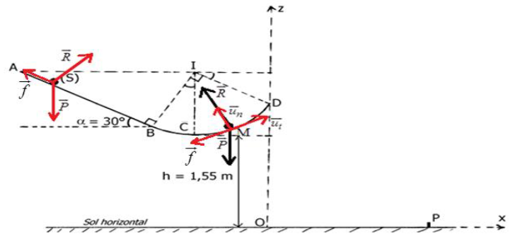
Le théorème de l'énergie cinétique s'écrit entre

$A\$ et

$\ D$

$E_{C_{D}}-E_{C_{A}}=W_{AD}(\vec{P})+W_{AD}(\vec{R})+W_{AD}(\vec{f})$

Donc,

$0-0=mgr\cos\theta+0+W_{AD}(\vec{f})$

Ce qui donne :

$W_{AD}(\vec{f})=-mgr\cos\theta$

Calcul

$W_{\vec{f}}$

$\begin{array}{rcl} W_{AD}(\vec{f})&=&-mgr\cos\theta\\\\&=&-50\cdot 10^{-3}\times 10\times 0.9\cos 60\\\\&=&-0.225\;J\end{array}$

b) Intensité de la force

$\vec{f}$

$\begin{array}{rcl} W_{AD}(\vec{f})=-f\left(AB+r\dfrac{\pi}{2}\right)&\Rightarrow&f=-\dfrac{W_{AD}(\vec{f})}{AB+r\dfrac{\pi}{2}}\\\\&\Rightarrow&f=-\dfrac{-0.225\,J}{1.6+0.9\times\dfrac{\pi}{2}}\\\\&\Rightarrow&f=0.075\;N\end{array}$

Exercice 2

1) Détermination des composantes de l'accélération de la bombe

$-\$ Système : la bombe

$-\$ Référentiel d'étude : terrestre supposé galiléen

$-\$ Bilan des forces appliquées :

$\overrightarrow{P}$

La relation fondamentale de la dynamique appliquée à la bombe s'écrit :

$\begin{array}{rcl}\overrightarrow{P}&=&m\overrightarrow{a}\\\Rightarrow\;m\overrightarrow{g}&=&m\overrightarrow{a}\\\Rightarrow\overrightarrow{a}&=&\overrightarrow{g}\\\Rightarrow\overrightarrow{a}\left\lbrace\begin{array}{rcl}a_{x}&=&0\\a_{y}&=&g \end{array}\right.\end{array}$

$\begin{array}{lcl}\dfrac{\mathrm{d}\overrightarrow{V}}{\mathrm{d}t}&=&\overrightarrow{a}\\ \Rightarrow\left\lbrace\begin{array}{rcl}V_{x}&=&cte\\V_{y}&=&gt+cte\end{array}\right.\end{array}$

$\left\lbrace\begin{array}{lllll}V_{x}(0)&=&cte&=&V_{0}\\V_{y}(0)&=&-g\times 0+cte&=&0 \end{array}\right.$

$\Rightarrow\overrightarrow{V}\left\lbrace\begin{array}{lcl}V_{x}&=&V_{0}\\V_{y}&=&gt \end{array}\right.$

$\dfrac{\mathrm{d}\overrightarrow{OM}}{\mathrm{d}t}=\overrightarrow{V}\Rightarrow\overrightarrow{OM}\left\lbrace\begin{array}{lcl}x&=&V_{0}t+cte\\y&=&\dfrac{1}{2}gt^{2}+cte \end{array}\right.$

$\left\lbrace\begin{array}{lllll}x(0)&=&V_{0}\times 0+cte&=&0\\y(0)&=&\dfrac{1}{2}g\times 0^{2}+cte&=&0 \end{array}\right.$

$\Rightarrow\overrightarrow{OM}\left\lbrace\begin{array}{lcl}x&=&V_{0}t\\y&=&\dfrac{1}{2}gt^{2} \end{array}\right.$

3) Équation de la trajectoire de la bombe

$x=v_{0}t\Rightarrow\;t=\dfrac{x}{v_{0}}$ et comme

$y=\dfrac{1}{2}gt^{2}$

$\Rightarrow\;y=\dfrac{1}{2}g\left(\dfrac{x}{v_{0}}\right)^{2}\Rightarrow\;y=\dfrac{1}{2}g\dfrac{x^{2}}{v_{0}^{2}}$

4) La position du véhicule par rapport à l'origine

$O$

Le théorème du centre d'inertie s'écrit :

$\begin{array}{lcl} y&=&\dfrac{1}{2}g\dfrac{x^{2}}{v_{0}^{2}}\\&=&2000\\\Rightarrow\;x^{2}&=&\dfrac{2v_{0}^{2}\times 2000}{g}\\\Rightarrow\;x&=&\sqrt{\dfrac{2v_{0}^{2}\times 2000}{g}}\\&=&\sqrt{\dfrac{2\times 400^{2}\times 2000}{10}}\\\Rightarrow\;x&=&8000\,m \end{array}$

Détermination de la date d'arrivée de la bombe au véhicule.

$t=\dfrac{x}{v_{0}}=\dfrac{8000}{400}\Rightarrow\;t=20s$

5) Position de l'avion à la date d'arrivée de la bombe au véhicule

$x=v_{0}t=400\times 20=8000\,m$

6) Détermination des caractéristiques du vecteur vitesse de la bombe à

$1000\,m$ au-dessus du sol.

$-\$ Direction : tangent à la trajectoire au point considéré

$-\$ Sens : dirigé vers le sol

$-\$ Valeur :

$\begin{array}{lcl} t&=&\dfrac{x}{v_{0}}\\&=&\dfrac{1000}{400}\\\Rightarrow\;t&=&2.5s\\\Rightarrow\;v&=&\sqrt{v_{x}^{2}(t=2.5s)+v_{y}^{2}(t=2.5s)}\\&=&\sqrt{400^{2}+(10\times 2.5)^{2}}\\\Rightarrow\;v&=&4.72\cdot 10^{2}m\cdot s^{-1} \end{array}$

Exercice 3

1) Calcul de la valeur de l'angle

$\alpha.$

$-\$ Système : La bille

$-\$ Référentiel d'étude : terrestre supposé galiléen

$-\$ Bilan des forces appliquées : le poids

$\overrightarrow{P}$ et la tension

$\overrightarrow{T}$ du fil

Le théorème de l'énergie cinétique entre

$M_{1}$ et

$M_{2}$ s'écrit :

$\begin{array}{lcl} E_{C_{M1}}-E_{C_{M1}}&=&W_{M1M2}(\overrightarrow{P})+W_{M1M2}(\overrightarrow{T})\\\Rightarrow\dfrac{1}{2}mv^{2}-0&=&mg(1-\cos\alpha)+0\\\Rightarrow\cos\alpha&=&1-\dfrac{v^{2}}{2gl}\\\Rightarrow\cos\alpha&=&1-\dfrac{3^{2}}{2\times 10\times 0.9}\\\Rightarrow\cos\alpha&=&0.5\\\alpha&=&60^{\circ} \end{array}$

2) Calcul la vitesse de la bille

La conservation de la quantité de mouvement :

$m_{1}\overrightarrow{v}+\overrightarrow{0}=m_{1}\overrightarrow{v'_{1}}+m_{2}\overrightarrow{v_{A}}$

Suivant le sens de

$\overrightarrow{v'_{1}}$ :

$\begin{array}{lcl} \Rightarrow\;m_{1}v'_{1}-m_{2}v_{A}&=&-m_{1}v\\\Rightarrow\;m_{1}v'_{1}&=&m_{2}v_{A}-m_{1}v\\\Rightarrow\;v'_{1}&=&v_{A}-v(m_{2}=m_{1})\\\Rightarrow\;v'_{1}&=&v_{A}-v\\&=&4-3\\\Rightarrow\;v'_{1}&=&1\,m\cdot s^{-1} \end{array}$

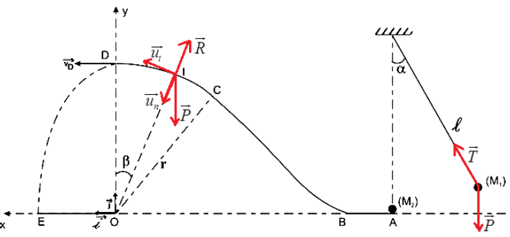
3) a) Expression, en fonction de

$g$ ,

$r$ ,

$\beta$ et

$v_{A}$ , de la vitesse de la bille

$M_{2}$ au point

$I$

$-\$ Système : Le pendule

$-\$ Référentiel d'étude : terrestre supposé galiléen

$-\$ Bilan des forces appliquées : le poids

$\overrightarrow{P}$

Le théorème de l'énergie cinétique entre

$A$ et

$I$ s'écrit :

$\begin{array}{lcl} E_{C_{M_{I}}}-E_{C_{M_{A}}}&=&W_{AI}(\overrightarrow{P})\\\Rightarrow\dfrac{1}{2}m_{2}v_{I}^{2}-\dfrac{1}{2}m_{2}v_{A}^{2}&=&-m_{2}gr\cos\beta\\\Rightarrow\;v_{I}&=&\sqrt{v_{A}^{2}-2gr\cos\beta} \end{array}$

b) Expression, en fonction de

$m_{2}$ ,

$g$ ,

$r$ ,

$\beta$ et

$v_{A}$ , de l'intensité de la réaction de la piste sur la bille

$M_{2}$ au point

$I$

Le théorème du centre d'inertie appliqué à la bille soumise à son poids et la réaction de la piste, dans le référentiel terrestre supposé galiléen, s'écrit :

$\overrightarrow{P}+\overrightarrow{R}=m_{2}\overrightarrow{a}$

Projection dans le repère de Frenet

$(I\;,\ \overrightarrow{u_{t}}\;,\ \overrightarrow{u_{n}})$ et suivant

$\overrightarrow{u_{n}}$ :

$\begin{array}{lcl} \Rightarrow\;m_{2}g\cos\beta-R&=&m_{2}\dfrac{v_{I}^{2}}{r}\\\Rightarrow\;R&=&m_{2}g\cos\beta-m_{2}\dfrac{v_{I}^{2}}{r}-m\\&=&m_{2}g\cos\beta-m_{2}\dfrac{v_{A}^{2}-2gr\cos\beta}{r}\\\Rightarrow\;R&=&m_{2}\left(3g\cos\beta-\dfrac{v_{A}^{2}}{r}\right) \end{array}$

c) Calcul de la valeur de

$r.$

$v_{I}=\sqrt{v_{A}^{2}-2gr\cos\beta}$

$\begin{array}{lcl} \text{En : }D\beta=0\\\Rightarrow\;v_{D}&=&\sqrt{v_{A}^{2}-2gr}\\\Rightarrow\;r&=&\dfrac{v_{A}^{2}-v_{D}^{2}}{2g}\\&=&\dfrac{4^{2}-1^{2}}{2\times 10}\\\Rightarrow\;r&=&0.75\,m \end{array}$

4) a) Équation cartésienne de la trajectoire de la bille

$M_{2}$

$-\$ Système : La bille

$-\$ Référentiel d'étude : terrestre supposé galiléen

$-\$ Bilan des forces appliquées : le poids

$\overrightarrow{P}$

Le théorème du centre d'inertie s'écrit :

$\begin{array}{lcl} \overrightarrow{P}&=&m\overrightarrow{a}\\\Rightarrow\;m\overrightarrow{g}&=&m\overrightarrow{a}\\\Rightarrow\overrightarrow{a}&=&\overrightarrow{g}\end{array}\\\Rightarrow\overrightarrow{a}\left\lbrace\begin{array}{lcl}a_{x}&=&0\\a_{y}&=&-g \end{array}\right.$

$\dfrac{\mathrm{d}\overrightarrow{V}}{\mathrm{d}t}=\overrightarrow{a}$

$\Rightarrow\overrightarrow{V}\left\lbrace\begin{array}{lcl}V_{x}&=&cte\\V_{y}&=&-gt+cte \end{array}\right.$

$\Rightarrow\overrightarrow{V}(t=0)\left\lbrace\begin{array}{lllll}V_{x}&=&cte&=&V_{D}\\V_{y}&=&-g\times 0+cte&=&0 \end{array}\right.$

$\Rightarrow\overrightarrow{V}\left\lbrace\begin{array}{lcl}V_{x}&=&V_{D}\\V_{y}&=&-gt \end{array}\right.$

$\dfrac{\mathrm{d}\overrightarrow{OM}}{\mathrm{d}t}=\overrightarrow{V}\Rightarrow\overrightarrow{OM}\left\lbrace\begin{array}{lcl}x&=&V_{D}t\\y&=&-\dfrac{1}{2}gt^{2}+R \end{array}\right.$

$\Rightarrow\overrightarrow{OM}(t=0)\left\lbrace\begin{array}{lllll}x&=&V_{D}\times 0+cte&=&0\\y&=&-\dfrac{1}{2}g\times 0^{2}+cte&=&r \end{array}\right.$

$\Rightarrow\overrightarrow{OM}\left\lbrace\begin{array}{lcl}x&=&V_{D}t\\y&=&-\dfrac{1}{2}gt^{2}+r \end{array}\right.$

$\begin{array}{lcl} x&=&v_{D}t\\\Rightarrow\;t&=&\dfrac{x}{v_{D}}\\\Rightarrow\;y&=&-\dfrac{1}{2}g\dfrac{x^{2}}{v_{D}^{2}}+r \end{array}$

b) Calcul de la distance

$OE$

La distance

$OE$ correspond à la portée ; donc :

$y=0$

$\begin{array}{lcl} \Rightarrow-\dfrac{1}{2}g\dfrac{x_{E}^{2}}{v_{D}^{2}}+r&=&0\\\Rightarrow\;x_{E}&=&\sqrt{\dfrac{2v_{D}^{2}r}{g}}\\&=&\sqrt{\dfrac{2\times 1^{2}\times 0.75}{10}}\\\Rightarrow\;x_{E}&=&0.39\,m \end{array}$

Exercice 4

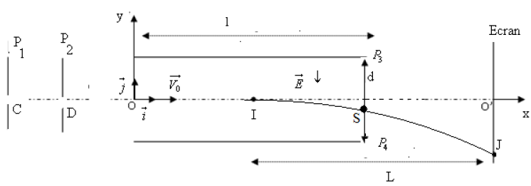
1. Signe de la tension

$U_{CD}$

Pour que les protons chargés positivement soient accélérés, il faut que les plaques

$P_{1}$ et

$P_{2}$ soient respectivement chargées positivement et négativement.

La tension

$U_{CD}$ est donc de signe positif

2.1 Expression de la vitesse d'un proton en

$D$ en fonction de

$U$ ,

$e$ et

$m_{p}$

$-\$ Système : le proton

$-\$ Référentiel d'étude : de laboratoire supposé galiléen

$-\$ Bilan des forces appliquées : le poids

$\overrightarrow{P}$ et la force électrique

$\overrightarrow{F}$

Le théorème de l'énergie cinétique appliqué à l'électron entre

$C$ et

$D$ s'écrit :

$\begin{array}{lcl} \Delta\,E_{C}&=&\sum\,W\\\Rightarrow\;E_{C_{O}}-E_{C_{D}}&=&W_{DO}(\overrightarrow{P})\text{ or }\overrightarrow{P}\perp\overrightarrow{DO}\\\Rightarrow\;W_{DO}(\overrightarrow{P})&=&0\\\Rightarrow\;E_{C_{O}}-E_{C_{D}}&=&0\\\Rightarrow\;E_{C_{O}}&=&E_{C_{D}}\\&=&\text{costante} \end{array}$

L'énergie cinétique se conserve donc entre

$D$ et

$O$

3.2 Équations du mouvement d'un proton

$-\$ Système : le proton

$-\$ Référentiel d'étude : de laboratoire supposé galiléen

$-\$ Bilan des forces appliquées : la force électrique

$\overrightarrow{F}$ et le poids

$\overrightarrow{P}$ négligeable devant la force électrique

$\overrightarrow{F}$

Le théorème du centre d'inertie s'écrit :

$\begin{array}{lcl} \overrightarrow{F}&=&m_{F}\overrightarrow{a}\\\Rightarrow\;e\overrightarrow{E}&=&m_{F}\overrightarrow{a}\\\Rightarrow\overrightarrow{a}&=&\dfrac{e\overrightarrow{E}}{m_{F}}\end{array}\\\Rightarrow\overrightarrow{a}\left\lbrace\begin{array}{lcl}a_{x}&=&0\\a_{y}&=&-\dfrac{eE}{m_{F}}\end{array}\right.$

$\dfrac{\mathrm{d}\overrightarrow{V}}{\mathrm{d}t}=\overrightarrow{a}$

$\Rightarrow\overrightarrow{V}\left\lbrace\begin{array}{lcl}v_{x}&=&cte\\v_{y}&=&-\dfrac{eE}{m_{F}}t+cte \end{array}\right.$

$\Rightarrow\overrightarrow{V}(t=0)\left\lbrace\begin{array}{lllll}v_{x}&=&cte&=&v_{D}\\v_{y}&=&-\dfrac{eE}{m_{F}}\times 0+cte&=&0 \end{array}\right.$

$\Rightarrow\overrightarrow{V}\left\lbrace\begin{array}{lcl}v_{x}&=&V_{D}\\v_{y}&=&-\dfrac{eE}{m_{F}}t \end{array}\right.$

$\dfrac{\mathrm{d}\overrightarrow{OM}}{\mathrm{d}t}=\overrightarrow{V}\Rightarrow\overrightarrow{OM}\left\lbrace\begin{array}{lcl}x&=&v_{D}t+cte\\y&=&-\dfrac{1}{2}\dfrac{eE}{m_{p}}t^{2}+cte \end{array}\right.$

$\Rightarrow\overrightarrow{OM}(t=0)\left\lbrace\begin{array}{lllll}x&=&v_{D}\times 0+cte&=&0\\y&=&-\dfrac{1}{2}\dfrac{eE}{m_{p}}\times 0^{2}+cte&=&0 \end{array}\right.$

$\Rightarrow\overrightarrow{OM}\left\lbrace\begin{array}{lcl}x&=&v_{D}t\\y&=&-\dfrac{1}{2}\dfrac{eE}{m_{p}}t^{2} \end{array}\right.$

3.3 Vérifions que l'équation de la trajectoire peut s'écrire :

$y=-\dfrac{U'}{4\mathrm{d}U}x^{2}$

$x=v_{D}t\Rightarrow\;t=\dfrac{x}{v_{D}}$

comme

$y=-\dfrac{1}{2}\dfrac{eE}{m_{p}}t^{2}$

$\Rightarrow\;y=-\dfrac{1}{2}\dfrac{eE}{m_{p}}\left(\dfrac{x}{v_{D}}\right)=-\dfrac{1}{2}\dfrac{eE}{m_{p}}\dfrac{x^{2}}{v_{D}^{2}}$ ;

$\begin{array}{lcl} \text{et omme }E=\dfrac{U'}{\mathrm{d}}\text{ et }v_{D}&=&\sqrt{\dfrac{2eE}{m_{p}}}\\\Rightarrow\;v_{D}^{2}&=&\dfrac{2eE}{m_{p}}\\\Rightarrow\;y&=&-\dfrac{1}{2}\dfrac{e}{m_{p}}\dfrac{U'}{\mathrm{d}}\dfrac{x^{2}}{\dfrac{2eU}{m_{p}}}\\\Rightarrow\;y&=&-\dfrac{1}{4}\dfrac{U'}{\mathrm{d}U}x^{2} \end{array}$

3.4 Les protons sortent du champ électrostatique

$\overrightarrow{E}$ sans heurter la plaque

$P_{4}$ si :

$y=-\dfrac{1}{4}\dfrac{U'}{\mathrm{d}U}l^{2}<-\dfrac{\mathrm{d}}{2}$

3.5 Détermination de

$U'$

Les protons sortent du champ par le point

$S$

$\begin{array}{lcl} y&=&-\dfrac{1}{4}\dfrac{U'}{\mathrm{d}U}l^{2}\\&=&-\dfrac{\mathrm{d}}{5}\\\Rightarrow\;U'&=&\dfrac{4\mathrm{d^{2}}}{5l^{2}}U\\&=&\dfrac{4\times 7^{2}}{5\times 20^{2}}\times 10^{3}\\\Rightarrow\;U'&=&9.8\cdot 10^{1}V \end{array}$

4.1 Représentation de la trajectoire (voir figure).

4.2 Expression littérale de la déviation

$O'J$ du spot sur l'écran.

$\begin{array}{lcl} \tan\alpha&=&\dfrac{O'J}{L}\\&=&\dfrac{y_{S}}{\dfrac{l}{2}}\\\Rightarrow\;O'J&=&\dfrac{2y_{S}L}{l}\\&=&\dfrac{-\dfrac{1}{4}\dfrac{U'}{\mathrm{d}U}l^{2}L}{l}U\\\Rightarrow\;O'J&=&-\dfrac{1}{4}\dfrac{U'l}{\mathrm{d}U}L\\&=&-\dfrac{1}{4}\times\dfrac{9.8\cdot 10^{1}\times 20}{7\times 10^{3}}\times 20\\\Rightarrow\;O'J&=&1.4\,cm \end{array}$

Exercice 5

1) Détermination des lois horaires du mouvement

$-\$ Système étudié : la bille

$-\$ Référentiel : terrestre supposé galiléen

$-\$ Bilan des forces appliquées : le poids P de la bille

$-\$ La deuxième de Newton s'écrit :

$\dfrac{\mathrm{d}\overrightarrow{V}}{\mathrm{d}t}=\overrightarrow{a}$

$\Rightarrow\overrightarrow{V}\left\lbrace\begin{array}{lcl}V_{x}&=&cte\\V_{y}&=&-gt+cte \end{array}\right.$

$\text{Or }\left\lbrace\begin{array}{lllll}V_{x}(0)&=&cte&=&V_{0}\sin\theta\\V_{y}(0)&=&-g\times 0+cte&=&V_{0}\cos\theta \end{array}\right.$

$\Rightarrow\overrightarrow{V}\left\lbrace\begin{array}{lcl}V_{x}&=&V_{0}\sin\alpha\\V_{y}&=&-gt+V_{0}\cos\alpha \end{array}\right.$

$\dfrac{\mathrm{d}\overrightarrow{OM}}{\mathrm{d}t}=\overrightarrow{V}\Rightarrow\overrightarrow{OM}\left\lbrace\begin{array}{lcl}x&=&(V_{0}\sin\alpha)t+cte\\y&=&-\dfrac{1}{2}gt^{2}+(V_{0}\cos\alpha)t+cte \end{array}\right.$

$\Rightarrow\left\lbrace\begin{array}{lllll}x(0)&=&V_{0}\times 0+cte&=&0\\y(0)&=&-\dfrac{1}{2}g\times 0^{2}+V_{0}\cos\alpha\times 0+cte&=&0 \end{array}\right.$

$\Rightarrow\overrightarrow{OM}\left\lbrace\begin{array}{lcl}x&=&(V_{0}\sin\alpha)t\quad(1)\\y&=&-\dfrac{1}{2}gt^{2}+(V_{0}\cos\alpha)t\quad(2) \end{array}\right.$

$(1)\qquad\Rightarrow\;x=(V_{0}\sin\alpha)t\Rightarrow\;t=\dfrac{x}{V_{0}\sin\alpha}$

$\text{Dans }(2)\Rightarrow\;y=-\dfrac{1}{2}g\left(\dfrac{x}{V_{0}\sin\alpha}{2}\right)^{2}+V_{0}\cos\alpha\times\dfrac{x}{V_{0}\sin\alpha}$

$\Rightarrow\;y=-\dfrac{1}{2}g\dfrac{x^{2}}{V_{0}^{2}\sin^{2}\alpha}+x\cot\,g\alpha$

3) a) Temps pendant lequel la bille s'élève avant de descendre

La composante

$V_{y}$ du vecteur vitesse est nulle

$\begin{array}{lcl} V_{y}&=&-gt+V_{0}\cos\alpha\\&=&0\\\Rightarrow\;t&=&\dfrac{V_{0}\cos\alpha}{g}\\&=&\dfrac{16\cos 50}{9.8}\\\Rightarrow\;t&=&1.0s\\\Rightarrow\;t&=&1.3s \end{array}$

b) Vitesse à la fin de cette phase ascendante

$\begin{array}{lcl} V&=&\sqrt{V_{x}^{2}+V_{y}^{2}}\\&=&\sqrt{V_{0}\sin^{2}\alpha+0}\\&=&V_{0}\sin\alpha\\&=&16\sin 50\\\Rightarrow\;V&=&12\,m\cdot s^{-1} \end{array}$

4) Altitude maximale atteinte par la bille

$y_{max}=-\dfrac{1}{2}gt^{2}+(V_{0}\cos\alpha)t$

$\text{or }t=\dfrac{V_{0}\cos\alpha}{g}\Rightarrow\;y_{max}=-\dfrac{1}{2}g\left(\dfrac{V_{0}\cos\alpha}{g}\right)^{2}+(V_{0}\cos\alpha)\times\dfrac{V_{0}\cos\alpha}{g}$

$\Rightarrow\;y_{max}=\dfrac{V_{0}\cos^{2}\alpha}{2g}=\dfrac{16^{2}\cos^{2}50}{2\times 9.8}$

$\Rightarrow\;y_{max}=5.4\,m$

5) a) Détermination de la distance

$OP$

C'est l'abscisse d'ordonnée nulle

$\begin{array}{lcl} y&=&\\\Rightarrow-\dfrac{1}{2}g\dfrac{x_{p}^{2}}{V_{0}^{2}\sin^{2}\alpha}+x_{p}\cot g\alpha&=&0\\\Rightarrow\;x_{p}\left(-\dfrac{1}{2}g\dfrac{x_{p}}{V_{0}^{2}\sin^{2}\alpha}+\cot g\alpha\right)&=&0\\\Rightarrow\;x_{p}&=&0\text{ (Origine O)} \end{array}$

$\begin{array}{lcl} \text{ou }x_{p}&=&\dfrac{2\cot g\alpha\times V_{0}^{2}\sin^{2}\alpha}{g}\\&=&\dfrac{2V_{0}^{2}\sin\alpha\cos\alpha}{g}\\&=&\dfrac{V_{0}^{2}\sin 2\alpha}{g}\\&=&\dfrac{16^{2}\sin(2\times 50)}{9.8}\\\Rightarrow\;x_{p}&=&25.7\,m \end{array}$

b) Valeur de

$\alpha$ pour laquelle

$OP$ est maximale

$x_{p}$ est maximale lorsque

$\sin 2\alpha=1\Rightarrow\;2\alpha=\dfrac{\pi}{2}\Rightarrow\alpha=\dfrac{\pi}{4}$

6) Montrons qu'il y a deux angles de tir

$\alpha_{1}$ et

$\alpha_{2}$ permettant d'atteindre

$Q$

$\begin{array}{lcl} y&=&\\\Rightarrow-\dfrac{1}{2}g\dfrac{x_{0}^{2}}{V_{0}^{2}\sin^{2}\alpha}+x_{0}\cot g\alpha&=&0\\\Rightarrow\;x_{0}&=&0\text{ ou }\dfrac{1}{2}g\dfrac{1}{V_{0}^{2}\sin^{2}\alpha}x_{0}-\cot g\alpha&=&0 \end{array}$

$\begin{array}{lcl} \text{Comme }\dfrac{1}{\sin^{2}\alpha}&=&1+\cot g^{2}\alpha\\\Rightarrow\dfrac{1}{2}(1+\cot g^{2}\alpha)g x_{0}-\cot g\alpha&=&0\\\Rightarrow\cot g^{2}\alpha-\dfrac{2V_{0}^{2}}{g x_{0}}\cot g\alpha+1&=&0\\\\\Rightarrow\cot g\alpha_{1}&=&\dfrac{\dfrac{V_{0}^{2}}{g x_{0}}-\sqrt{\dfrac{V_{0}^{4}}{(g x_{0})^{2}}-1}}{1}\\&=&\dfrac{V_{0}^{2}}{g x_{0}}-\sqrt{\dfrac{V_{0}^{4}}{(g x_{0})^{2}}-1}\\&=&\dfrac{16^{2}}{9.8\times 10}-\sqrt{\dfrac{16^{4}}{(9.8\times 10)^{2}}-1}\\\Rightarrow\cot g\alpha_{1}&=&0.20\\\\\Rightarrow\cot g\alpha_{2}&=&\dfrac{\dfrac{V_{0}^{2}}{g x_{0}}+\sqrt{\dfrac{V_{0}^{4}}{(g x_{0})^{2}}-1}}{1}\\&=&\dfrac{V_{0}^{2}}{g x_{0}}+\sqrt{\dfrac{V_{0}^{4}}{(g x_{0})^{2}}-1}\\&=&\dfrac{16^{2}}{9.8\times 10}+\sqrt{\dfrac{16^{4}}{(9.8\times 10)^{2}}-1}\\\Rightarrow\cot g\alpha_{2}&=&5.03 \end{array}$

$\alpha_{1}=7807^{\circ}\text{ et }\alpha_{2}=11.3^{\circ}$

Exercice 6

I. La trajectoire balistique de

$C$ vers

$T$

a) Un référentiel galiléen est un référentiel dans le lequel le principe de l'inertie est vérifié.

b) Bilan des forces qui s'exercent sur la balle

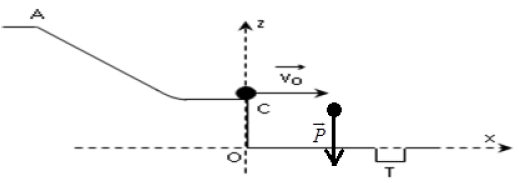
Le poids de la balle est la seule force qui s'exerce sur la balle.

La balle tombe en chute libre

c) Équations horaires de la vitesse et de la position de la balle

$B.$

$-\$ Système étudié : la bille

$-\$ Référentiel : terrestre supposé galiléen

$-\$ Bilan des forces appliquées : le poids

$\overrightarrow{P}$ de la balle

Le théorème du centre d'inertie s'écrit :

$\Rightarrow\overrightarrow{V}\left\lbrace\begin{array}{lcl}V_{x}&=&V_{0}\\V_{z}&=&-gt \end{array}\right.$

$\Rightarrow\overrightarrow{OM}\left\lbrace\begin{array}{lcl}x&=&V_{0}t\quad(1)\\z&=&-\dfrac{1}{2}gt^{2}+z_{C}\quad(2) \end{array}\right.$

d) Équation

$z(x)$ de la trajectoire de la balle

$B.$

$(1)\qquad\Rightarrow\;x=V_{0}t\Rightarrow\;t=\dfrac{x}{V_{0}}$

$\text{Dans }(2)\Rightarrow\;z=-\dfrac{1}{2}g\left(\dfrac{x}{V_{0}}\right)^{2}+z_{C}$

$\Rightarrow\;z=-\dfrac{1}{2}g\dfrac{x^{2}}{V_{0}^{2}}+z_{C}$

e) Abscisse

$x_{T}$ du trou

$T$ pour que la balle tombe directement dedans

La balle tombe dans lorsque :

$\begin{array}{lcl}z&=&0\\\Rightarrow-\dfrac{1}{2}g\dfrac{x_{T}^{2}}{V_{0}^{2}}+z_{C}&=&0\\\Rightarrow\;x_{T}^{2}&=&\dfrac{2z_{C}V_{0}^{2}}{g}\\\\\Rightarrow\;x_{T}&=&\sqrt{\dfrac{2z_{C}V_{0}^{2}}{g}}\\&=&\sqrt{\dfrac{2\times 40\cdot 10^{-2}\times 2.0}{9.8}}\\\Rightarrow\;x_{T}&=&0.40\,m \end{array}$

f) Détermination la date

$t_{F}$ à laquelle la balle B tombe dans le trou

$\begin{array}{lcl}z&=&-\dfrac{1}{2}gt^{2}+z_{C}\\&=&0\\\Rightarrow\;t^{2}&=&\dfrac{2z_{C}}{g}\\\Rightarrow\;t&=&\sqrt{\dfrac{2z_{C}}{g}}\\&=&\sqrt{\dfrac{2\times 40\cdot 10^{-2}}{9.8}}\\\Rightarrow\;t&=&2.8s \end{array}$

II. Le mouvement sur la rampe

a) Détermination la hauteur

$z_{A}$ de

$A$ nécessaire pour que la balle arrive en

$C.$

Le théorème de l'énergie cinétique appliqué à la balle entre

$A$ et

$C$

$\begin{array}{lcl} E_{C_{C}}-E_{C_{A}}&=&W_{\overrightarrow{AC}}(\overrightarrow{P})\\\Rightarrow\dfrac{1}{2}mV_{C}^{2}-\dfrac{1}{2}mV_{A}^{2}&=&mg(z_{A}-z_{C})\\\\\Rightarrow\;z_{A}&=&\dfrac{1}{2g}(V_{C}^{2}-V_{A}^{2})+z_{C}\\&=&\dfrac{1}{2\times 9.8}(2.0^{2}-0.80^{2})+40\cdot 10^{-2}\\\Rightarrow\;z_{A}&=&57\,cm \end{array}$

b) la vitesse est horizontale du fait qu'elle est tangente à la trajectoire au point

$C.$

Exercice 7

1) a) Montrons que la trajectoire est plane

$-\$ Système : La balle

$-\$ Référentiel d'étude : terrestre supposé galiléen

$-\$ Bilan des forces appliquées : le poids

$\overrightarrow{P}$

Le théorème du centre d'inertie s'écrit :

$\dfrac{\mathrm{d}\overrightarrow{V}}{\mathrm{d}t}=\overrightarrow{a}$

$\Rightarrow\overrightarrow{V}\left\lbrace\begin{array}{lcl}v_{x}&=&cte\\v_{y}&=&-gt+cte\\v_{z}&=&cte \end{array}\right.$

$\overrightarrow{V}(t=0)\left\lbrace\begin{array}{lllll}v_{x}&=&cte&=&v_{0}\cos\alpha\\v_{y}&=&-g\times 0+cte&=&v_{0}\sin\alpha\\v_{z}&=&cte&=&0 \end{array}\right.$

$\Rightarrow\overrightarrow{V}\left\lbrace\begin{array}{lcl}v_{x}&=&v_{0}\cos\alpha\\v_{y}&=&-gt+v_{0}\sin\alpha\\v_{z}&=&0 \end{array}\right.$

$\dfrac{\mathrm{d}\overrightarrow{OM}}{\mathrm{d}t}=\overrightarrow{V}\Rightarrow\overrightarrow{OM}\left\lbrace\begin{array}{lcl}x&=&(v_{0}\cos\alpha)t+cte\\y&=&-\dfrac{1}{2}gt^{2}+(v_{0}\sin\alpha)t+cte\\z&=&cte \end{array}\right.$

$\Rightarrow\overrightarrow{OM}(t=0)\left\lbrace\begin{array}{lllll}x&=&(v_{0}\cos\alpha)\times 0+cte&=&0\\y&=&-\dfrac{1}{2}g\times 0^{2}+(v_{0}\sin\alpha)\times 0+cte&=&h\\z&=&cte&=&0 \end{array}\right.$

$\Rightarrow\overrightarrow{OM}\left\lbrace\begin{array}{lcl}x&=&(v_{0}\cos\alpha)t\\y&=&-\dfrac{1}{2}gt^{2}+(v_{0}\sin\alpha)t+h\\z&=&0 \end{array}\right.$

$(1)\qquad\Rightarrow\;x=(V_{0}\sin\alpha)t\Rightarrow\;t=\dfrac{x}{V_{0}\sin\alpha}$

$\text{Dans }(2)\Rightarrow\;y=-\dfrac{1}{2}g\left(\dfrac{x}{V_{0}\sin\alpha}\right)^{2}+V_{0}\cos\alpha\times\dfrac{x}{V_{0}\sin\alpha}$

$\Rightarrow\;y=-\dfrac{1}{2}g\dfrac{x^{2}}{V_{0}^{2}\sin^{2}\alpha}+x\cot\,g\alpha$

Quelque soit

$t$ ,

$z=0$ , la trajectoire est plane et se fait dans le plan

$(xOy)$

b) Équation de cette trajectoire

On obtient cette équation en éliminant

$t$ entre

$x$ et

$y$ :

$\begin{array}{lcl} x&=&(v_{0}\cos\alpha)t\\\Rightarrow\;t&=&\dfrac{x}{v_{0}\cos\alpha}\\\Rightarrow\;y&=&-\dfrac{1}{2}g\left(\dfrac{x}{v_{0}\cos\alpha}\right)^{2}+(v_{0}\sin\alpha)\left(\dfrac{x}{v_{0}\cos\alpha}\right)+h\\\\\Rightarrow\;y&=&-\dfrac{1}{2}g\dfrac{x^{2}}{v_{0}^{2}\cos^{2}\alpha}+(\tan\alpha)x+h \end{array}$

c) Valeur de

$V_{0}$ pour que le panier soit réussi

Le panier est réussi si

$x=7.1\,m$ et

$y=3\,m$

$\begin{array}{lcl} y&=&-\dfrac{1}{2}g\dfrac{x^{2}}{v_{0}^{2}\cos^{2}\alpha}+(\tan\alpha)x+h\\\Rightarrow\;v_{0}^{2}&=&\dfrac{gx^{2}}{2\cos^{2}\alpha(x\tan\alpha+h-y)}\\\\\Rightarrow\;v_{0}&=&\sqrt{\dfrac{gx^{2}}{2\cos^{2}\alpha(x\tan\alpha+h-y)}}\\&=&\sqrt{\dfrac{10\times 7.1^{2}}{2\cos^{2}45^{\circ}(7.1\times\tan 45^{\circ}+2-3)}}\\\Rightarrow\;v_{0}&=&12\,m\cdot s^{-1} \end{array}$

d) Durée du trajet effectué par le ballon du point

$A$ au point

$C$

$\begin{array}{lcl} x&=&(v_{0}\cos\alpha)t\\\Rightarrow\;t&=&\dfrac{x}{v_{0}\cos\alpha}\\&=&\dfrac{7.1}{12\times\cos 45}\\\Rightarrow\;t&=&0.84s \end{array}$

2) Vérifions si le panier sera marqué ou non

$\begin{array}{lcl} x=0.9\Rightarrow\;x&=&-\dfrac{1}{2}10\times\dfrac{0.9^{2}}{12^{2}\times\cos^{2}45^{\circ}}+\tan 45^{\circ}\times 0.9+2\\\Rightarrow\;y&=&2.84\,m>2.7\,m \end{array}$

Le panier sera marqué

Exercice 8

Partie A

1) a) Représentation des forces qui s'exercent sur le solide.

b) Expression de l'accélération

$a$ du solide

$(S_{1})$

$-\$ Système : Le solide

$(S_{1})$

$-\$ Référentiel d'étude : terrestre supposé galiléen

$-\$ Bilan des forces appliquées : le poids

$\overrightarrow{P}$ et la réaction

$\overrightarrow{R}$ du plan.

Le théorème du centre d'inertie s'écrit :

$\overrightarrow{P}+\overrightarrow{R}=m_{1}\overrightarrow{a}$

Projection suivant l'axe

$x'x$ :

$m_{1}g\sin\alpha=10\times\sin 30\Rightarrow\alpha=5\,m\cdot s^{-2}$

Le mouvement du solide

$(S_{1})$ est uniformément accéléré

Calcul de

$a$ :

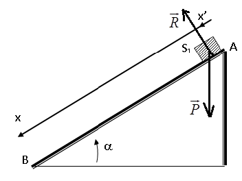
$a=g\sin\alpha=10\times\sin 30\Rightarrow\;a=5\,m\cdot s^{-2}$

2) a) Calcul de la valeur de la vitesse

$V_{B}$

$\begin{array}{lcl} V_{B}^{2}-V_{A}^{2}&=&2aAB\\\Rightarrow\;V_{B}^{2}-0&=&2aAb\\\Rightarrow\;V_{B}&=&\sqrt{2aAb}\\&=&\sqrt{2\times 5\times 2.5}\\\Rightarrow\;V_{B}&=&5\,m\cdot s^{-1} \end{array}$

b) Calcul de la durée

$t_{B}$ du trajet

$AB$

$V_{B}=at_{B}\Rightarrow\;t_{B}=\dfrac{V_{B}}{a}=\dfrac{5}{5}$

$\Rightarrow\;t_{B}=1s$

Partie B

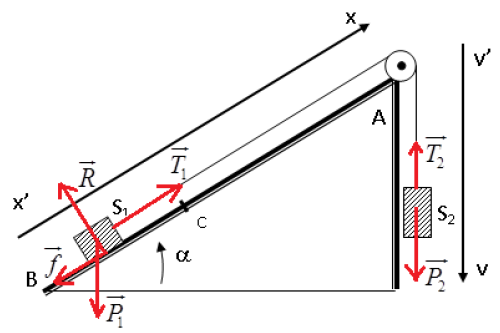
1) a) Expression de l'accélération

$a$ du système

La deuxième loi de Newton s'écrit :

$-\$ Pour le solide

$(S_{1})$ :

$\overrightarrow{f}+\overrightarrow{P_{1}}+\overrightarrow{R}+\overrightarrow{T_{1}}=m_{1}\overrightarrow{a_{1}}$

$x'x$ :

$-f-m_{1}g\sin\alpha+0+T_{1}=m_{1}a_{1}\Rightarrow\;T_{1}=m_{1}g\sin\alpha+m_{1}a_{1}$

$-\$ Pour le solide

$(S_{2})$ :

$\overrightarrow{P_{2}}+\overrightarrow{T_{2}}=m_{2}\overrightarrow{a_{2}}$

$y'y$ :

$m_{2}g-T_{2}=m_{2}a_{2}\Rightarrow\;T_{2}=m_{2}g-m_{2}a_{2}$

Les forces de frottement sont négligeables au niveau de la poulie :

$T_{1}=T'_{1}=T_{2}=T'_{2}$

$\Rightarrow\;m_{1}g\sin\alpha+m_{1}a_{1}+f=m_{2}g-m_{2}a_{2}$

Le fil est inextensible, l'accélération est la même en tout du fil :

$a_{1}=a_{2}=a$

$\Rightarrow(m_{1}+m_{2})a=(m_{2}-m_{1}\sin\alpha)g-f$

$\Rightarrow\;a=\dfrac{(m_{2}-m_{1}\sin\alpha)g-f}{(m_{1}+m_{2})}$

$m_{2}=m_{1}\Rightarrow\;a=\dfrac{m_{1}(1-\sin\alpha)g-f}{2m_{1}}$

$\Rightarrow\;a=(1-\sin\alpha)g-\dfrac{f}{2m_{1}}$

b) Calcul de

$a$

$\begin{array}{lcl} a&=&(1-\sin\alpha)g-\dfrac{f}{2m_{1}}\\&=&(1-\sin 30^{\circ})\times 10-\dfrac{0.2}{2\times 200\cdot 10^{-3}}\\\Rightarrow\;a&=&4.5\,m\cdot s^{-2} \end{array}$

2) Calcul de

$v_{C}$

$v_{C}=at_{C}=4.5\times 1\Rightarrow\;v_{C}=4.5\,m\cdot s^{-1}$

3) a) Expression de la nouvelle accélération

$a_{1}$ du solide

$(S_{1})$ après la coupure du fil

La deuxième loi de Newton s'écrit :

$\overrightarrow{f}+\overrightarrow{P_{1}}+\overrightarrow{R}=m_{1}\overrightarrow{a_{1}}$

$x'x$ :

$\begin{array}{lcl} f-m_{1}g\sin\alpha+0&=&m_{1}a_{1}\\\Rightarrow\;a_{1}&=&\dfrac{f-m_{1}g\sin\alpha}{m_{1}}\\\Rightarrow\;a_{1}&=&\dfrac{f}{m_{1}}-g\sin\alpha \end{array}$

Le mouvement du solide

$(S_{1})$ est uniformément varié

b) Calcul de la distance maximale

$($ par rapport au point

$C)$ parcourue par le solide

$(S_{1})$

$\begin{array}{lcl} 0^{2}-v_{C}^{2}&=&2a_{1}d\\\Rightarrow\;d&=&\dfrac{-v_{C}^{2}}{2a_{1}}\\\\&=&\dfrac{-v_{C}^{2}}{2\left(\dfrac{f}{m_{1}}-g\sin\alpha\right)}\\\\&=&\dfrac{-4.5^{2}}{2\left(\dfrac{0.2}{200\cdot 10^{-3}}-10\sin 30^{\circ}\right)}\\\Rightarrow\;d&=&2.5\,m \end{array}$

Exercice 9

I. 1) a) Expression littérale des lois horaires

$x(t)$ et

$z(t)$ du mouvement de la balle

Système étudié : la balle

Référentiel d'étude : terrestre supposé galiléen

Bilan des forces appliquées :

$\overrightarrow{P}$

Le théorème du centre d'inertie s'écrit :

$\begin{array}{lcl}\overrightarrow{P}&=&m\vec{a}\\\\\Rightarrow\,m\vec{g}&=&m\vec{a}\\\\\Rightarrow\vec{a}&=&\vec{g}\\\\&\Rightarrow&\vec{a}\left\lbrace\begin{array}{lcl}a_{x}&=&0\\a_{z}&=&-g \end{array}\right. \\\\&\Rightarrow&\vec{v}\left\lbrace\begin{array}{lcl}v_{x}&=&v_{0}\cos\alpha\\v_{z}&=&-gt+v_{0}\sin\alpha\end{array}\right.\\\\&\Rightarrow&\overrightarrow{OM}\left\lbrace\begin{array}{lcl}x&=&\left(v_{0}\cos\alpha\right)t\\\\z&=& -\dfrac{1}{2}gt^{2}+\left(v_{0}\sin\alpha\right)t+h\end{array}\right.\end{array}$

b) Équation de la trajectoire de la balle

$x=\left(v_{0}\cos\alpha\right)t$ ;

$z=-\dfrac{1}{2}gt^{2}+\left(v_{0}\sin\alpha\right)t+h$

En éliminant t entre les deux équations, il vient :

$\begin{array}{lcl} x&=&\left(v_{0}\cos\alpha\right)t\\\\\Rightarrow\,t&=&\dfrac{x}{v_{0}\cos\alpha}\\\\\Rightarrow\,z&=&-\dfrac{1}{2}g\left(\dfrac{x}{v_{0}\cos\alpha}\right)^{2}+\left(v_{0}\sin\alpha\right)\dfrac{x}{v_{0}\cos\alpha}+h\\\\\Rightarrow\,z&=&-\dfrac{1}{2}g\dfrac{x^{2}}{v_{0}^{2}\cos^{2}\alpha}+x\tan\alpha+h \end{array}$

2) Calcul des coordonnées du point

$S$ le plus élevé atteint par la balle.

Lorsque la balle atteint le point

$S$ le plus élevé, la vitesse se réduit à sa composante horizontale

$\begin{array}{lcl} v_{z}&=&-gt_{S}+v_{0}\sin\alpha\\\\&=&0\\\\\Rightarrow\,t_{S}&=&\dfrac{v_{0}\sin\alpha}{g}\\\\&\Rightarrow&\overrightarrow{OS}\left\lbrace\begin{array}{lcl} x&=&\dfrac{v_{0}^{2}\cos\alpha\sin\alpha}{g}\\\\ z&=&-\dfrac{1}{2}\dfrac{v_{0}^{2}\sin^{2}\alpha}{g}+\dfrac{v_{0}^{2}\sin^{2}\alpha}{g}+h \end{array}\right. \\\\&\Rightarrow&\overrightarrow{OS}\left\lbrace\begin{array}{lcl} x&=&\dfrac{v_{0}^{2}\cos\alpha\sin\alpha}{g}\\\\ z&=&\dfrac{1}{2}\dfrac{v_{0}^{2}\sin^{2}\alpha}{g}+h \end{array}\right. \\\\&\Rightarrow&\overrightarrow{OS}\left\lbrace\begin{array}{lcl} x&=&\dfrac{10^{2}\cos 45\sin 45}{9.8}\\\\ z&=&\dfrac{1}{2}\dfrac{10^{2}\sin^{2}45}{9.8}+2.7 \end{array}\right. \\\\ú&\Rightarrow&S\;(5.1m\ ;\ 5.3m) \end{array}$

$z=-\dfrac{1}{2}g\dfrac{x^{2}}{v_{0}^{2}\cos^{2}\alpha}+x\tan\alpha+h$

$\begin{array}{lcl} \alpha&=&0\\\\\Rightarrow\,z&=&-\dfrac{1}{2}g\dfrac{x^{2}}{v_{1}^{2}\cos^{2}0}+x\tan\,0+h\\\\\Rightarrow\,z&=&-\dfrac{1}{2}g\dfrac{x^{2}}{v_{1}^{2}}+h \end{array}$

2) Vérifions si la balle franchira le filet oui ou non

$\begin{array}{lcl} z(1)&=&-\dfrac{1}{2}g\dfrac{l^{2}}{v_{2}^{1}}+h\\\\&=&-\dfrac{1}{2}\times 10\times\dfrac{12^{2}}{25^{2}}+2.7\\\\\Rightarrow\,z(1)&=&1.55m>h_{0}\\\\&=&1m \end{array}$

la balle a franchi le filet.

3) Distance derrière le filet où retombe la balle sur le sol.

$\begin{array}{lcl} z&=&-\dfrac{1}{2}g\dfrac{x^{2}}{v_{1}^{2}}+h\\\\&=&0\\\\\Rightarrow\,x_{p}&=&\sqrt{\dfrac{2v_{1}^{2}h}{g}}\\\\&=&\sqrt{\dfrac{2\times 25^{2}\times 2.7}{9.8}}\\\\\Rightarrow\,x_{p}&=&18.6m \end{array}$

$\begin{eqnarray} d&=&x_{p}-l\nonumber\\\\&=&186-12\nonumber\\\\\Rightarrow\,d&=&66m \end{eqnarray}$

Auteur:

Amary Thiam & Sidy Mouhamed Ndiaye

Commentaires

Mamadi DIANE (non vérifié)

mer, 11/11/2020 - 12:35

Permalien

Remerciements

Bonjour Messieurs, Je vous adresse du fond du cœur mes remerciements. Ces documents m'ont été d'un grand support. Merci à vous. Que DIEU vous le rende.

répondre

Yousouf Traoré (non vérifié)

mer, 12/02/2020 - 18:31

Permalien

exo et leur correction

J'aime beaucoup cette page ça m'as beaucoup aider lors des exercices

répondre

Pape (non vérifié)

dim, 12/06/2020 - 22:40

Permalien

Remerciements

Merci

répondre

kheuch dady gueye (non vérifié)

dim, 01/17/2021 - 00:23

Permalien

avoir mon bac

en essayant de faire les exercices proposes ici et de les comprendre

répondre

Anonyme (non vérifié)

lun, 02/22/2021 - 20:17

Permalien

Très important

répondre

Thierno fall (non vérifié)

lun, 03/08/2021 - 12:37

Permalien

Erreur ou j’ai pas compris

Au niveau des équations horaires je crois que y’a erreur On doit avoir normalement 1/2 axt2 + voxt + xo 1/2 ayt2 + voyt + yo Si pouvez m’éclaircir cela svp ?

répondre

Thierno (non vérifié)

lun, 03/08/2021 - 12:49

Permalien

J’ai vu désolé

répondre

ianja (non vérifié)

ven, 03/26/2021 - 20:36

Permalien

pourquoi dans exo 1 TEC au pt

pourquoi dans exo 1 TEC au pt c et d sont d'angle 60

répondre

Abdoul Ndiaye (non vérifié)

dim, 04/18/2021 - 01:12

Permalien

Améliorer ma compréhension

En faisant beaucoup d exercices. Je veux la correction pour mieux comprendre et assumiler la démarche

répondre

Zaranada Venance (non vérifié)

jeu, 05/20/2021 - 13:50

Permalien

Physque

rien

répondre

Mohamed sidi be... (non vérifié)

dim, 10/24/2021 - 02:04

Permalien

Etudiant

Université de nouakcott

répondre

Amar Diaw (non vérifié)

dim, 12/26/2021 - 20:15

Permalien

Demande

S'il vous plaît !pour l'exercice 1 lorsqu'on cherche OP j'ai du mal à comprendre et j'ai essayé une autre méthode mais j'ai pas le même résultat que vous