
Corrigé Bac pc 1er groupe S1 S3 2017
Exercice 1
1.1. .
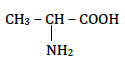
1.1.1. Nom officiel de la leucine : acide 2-amino-4-méthylpentanoique
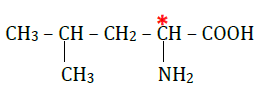
La molécule de leucine est chirale car elle possède un seul atome de carbone asymétrique (marqué ci-dessus).
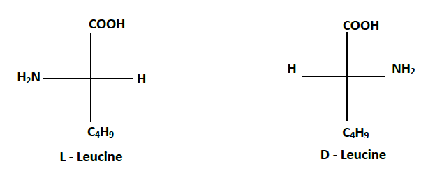
1.1.2. Représentations de Fischer :
1.2. .
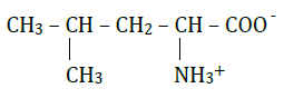
1.2.1. L'amphion :
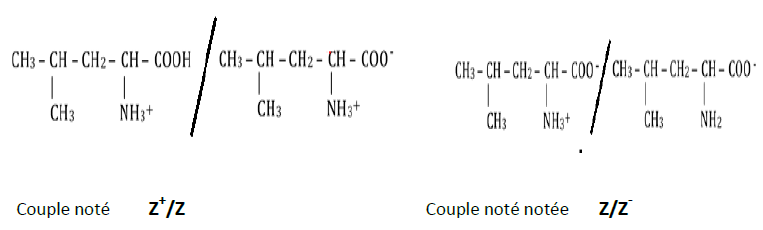
1.2.2. Les couples associés à l'amphion
1.2.3.1 Expression du $pH_{i}$ :
Posons $pk_{a1}=pk_{a}(Z^{+}/Z)\ $ et $\ pk_{a2}=pk_{a}(Z/Z^{-})$
Le $pH$ d'une solution quelconque d'isoleucine vérifie les relations suivantes :
On a : $$pH=pk_{a1}+\log\dfrac{[Z]}{[Z^{+}]}\quad(1)\quad\text{et}\quad pH=pk_{a2}+\log\dfrac{[Z^{-}]}{[Z]}\quad(2)$$
$\begin{array}{rcl} (1)+(2)\ \Rightarrow\ 2pH&=&pk_{a1}+pk_{a2}+\log\dfrac{[Z]}{[Z^{+}]}+\log\dfrac{[Z^{-}]}{[Z]}\\ \\&=&pk_{a1}+pk_{a2}+\log\dfrac{[Z^{-}]}{[Z^{+}]}\end{array}$
Au point isoélectrique on a :
$\begin{array}{lrcl}&[Z^{-}]&=&[Z^{+}]\\ \\ \Rightarrow&\dfrac{[Z^{-}]}{[Z^{+}]}&=&1\\ \\ \Rightarrow&\log\dfrac{[Z^{-}]}{[Z^{+}]}&=&0\\ \\ \Rightarrow&2pH_{i}&=&pk_{a1}+pk_{a2}\\ \\ \Rightarrow&pH_{i}&=&\dfrac{1}{2}(pk_{a1}+pk_{a2})\end{array}$
Ainsi, La valeur du $pH_{i}$ ne dépend pas de la concentration de l'acide $\alpha-\text{aminé}.$
1.2.3.2 Valeur du $pk_{a1}$ sachant que $pk_{a2}=9.6$
$\begin{array}{lrcl}&pH_{i}&=&\dfrac{1}{2}(pk_{a1}+pk_{a2})\\ \\ \Rightarrow&pk_{a1}&=&2pH_{i}-pk_{a2}\\& &=&2\times 6-9.6\\& &=&2.4\end{array}$
1.3. .
1.3.1.
$\begin{array}{lrcl} &M(A)+M(\text{Leucine)}&=&M(\text{(dipeptide)}+M(H_{2}O)\\ \Rightarrow&M(R)+205&=&202+18\\ \Rightarrow&M(R)&=&15\;g.mol^{-1}\end{array}$
$R$ est le radical méthyl $-CH_{3}.$
La formule semi-développée de $A$ est alors :
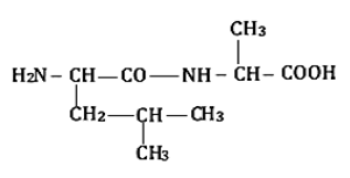
1.3.2. Formule semi-développée du dipeptide et étapes de sa synthèse :
Formule semi-développée du dipeptide
Les étapes de la synthèse du dipeptide :
$\lozenge\ $ Bloquer le groupe amino de la leucine et le groupe carboxyle de A.
$\lozenge\ $ Activer le groupe carboxyle de la leucine et le groupe amino de A.
$\lozenge\ $ Faire réagir les deux composés obtenus ci-dessus.
$\lozenge\ $ Après réaction, débloquer les groupements amino et carboxyle qui étaient bloqués.
Exercice 2
2.1. Équation-bilan :
$$\left.\begin{array}{rcl} 2\times[MnO_{4}^{-}+H^{+}+5e^{-}&\longrightarrow&Mn^{2+}+4H_{2}O]\\ 5\times[H_{2}O_{2}&\longrightarrow&O_{2} + 2H^{+} + 2e^{-}]\end{array}\right\rbrace$$
$$\Rightarrow\ 2MnO_{4}^{-} + 5H_{2}0_{2} + 6H_{3}O^{+}\ \longrightarrow\ 2Mn^{2+} + 5O_{2} + 14H_{2}0$$
ou encore $$2MnO_{4}^{-} + 5H_{2}0_{2} + 6H^{+}\ \longrightarrow\ 2Mn^{2+} + 5O_{2} + 8H_{2}0$$
2.2. Définition : la vitesse volumique de disparition de l'eau oxygénée est l'opposée de la dérivée par rapport au temps de la concentration molaire volumique de l'eau oxygénée : $$V=-\dfrac{dC}{dt}=-\dfrac{d[H_{2}O_{2}]}{dt}$$
Sa valeur est déterminée à partir du coefficient directeur de la tangente à la courbe à la date considérée : $$V(t=0)=V_{0}\approx 0.30\;mmol.L^{-1}.min^{-1}\quad\text{(graphiquement)}$$
2.3. Temps de demi-réaction $t_{\dfrac{1}{2}}$ :
$\begin{array}{lrcl} &[H_{2}O_{2}]_{t_{\frac{1}{2}}}&=&\dfrac{[H_{2}O_{2}]_{0}}{2}\\ & &=&3\;mmol.L^{-1}\\ \Rightarrow&t_{\frac{1}{2}}&\approx&14\;min\quad\text{(graphiquement)}\end{array}$
Vitesse $V_{\frac{1}{2}}=0.147\;mmol.L^{-1}.min^{-1}$ (graphiquement).
2.4. La vitesse diminue au cours du temps car la concentration du réactif diminue.
2.5. .
2.5.1.
$\begin{array}{lrcl} &V&=&-\dfrac{dC}{dt}\quad\text{or }\ C=C_{0}\mathrm{e}^{-kt}\\ \Rightarrow&\dfrac{dC}{dt}&=&-kC_{0}\mathrm{e}^{-kt}\\ \Rightarrow&V&=&kC_{0}\mathrm{e}^{-kt}\end{array}$
2.5.2. Valeur de $k$ :
$\begin{array}{lrcl} &V(t=0)&=&V_{0}\\& &=&kC_{0}\mathrm{e}^{0}\\& &=&kC_{0}\\ \Rightarrow&k&=&\dfrac{V_{0}}{C_{0}}\end{array}$
A.N : $k=\dfrac{0.3}{6}=0.05\;min^{-1}$
Relation simple entre $V\ $ et $\ C$ :
$\begin{array}{lrcl} &V&=&kC_{0}\mathrm{e}^{-kt}\quad\text{or }\ C=C_{0}\mathrm{e}^{-kt}\\ \Rightarrow&V&=&k.C\\& &=&0.05\times C\end{array}$
Valeur de $V(t=14\;min)$ :
$V_{t=14\;min}=0.05\times 3=0.15\;mmol.L^{-1}.min^{-1}$
Exercice 3
3.1. .
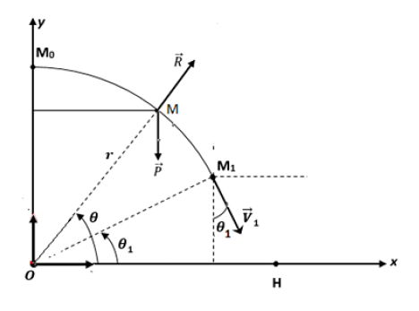
3.1.1. Bilan des forces : poids $\vec{P}\ $ et $\ \vec{R}$ réaction
3.1.2. TCI : $\vec{P}+\vec{R}=m\vec{a}$
Projetons suivant la normale : $P_{N}+R_{N}=a_{N}$
$\begin{array}{lrcl}\Rightarrow&m.g.\sin\theta-R&=&m.a_{N}\quad\text{or } a_{N}=\dfrac{V^{2}}{r}\\ \Rightarrow&R&=&m\left(g.\sin\theta-\dfrac{V^{2}}{r}\right)\end{array}$
3.1.3.
$\begin{array}{lcrcl} \text{T.E.C}&\Rightarrow&E_{c(M)}-E_{c(M_{0})}&=&W_{\vec{P}}+W_{\vec{R}}\\ &\Rightarrow&\dfrac{1}{2}mV^{2}&=&mgh\quad\text{avec }\ h=r(1-\sin\theta)\\ &\Rightarrow&\dfrac{1}{2}mV^{2}&=&mgr(1-\sin\theta)\\ &\Rightarrow&V^{2}&=&2.g.r(1-\sin\theta)\end{array}$
3.1.4. Lorsque le mobile quitte la piste en $M_{1}$ : $\theta=\theta_{1}\;;\ V=V_{1}\ $ et $\ R=0$
$\begin{array}{lrcl}\Rightarrow&m\left(g.\sin\theta-\dfrac{V^{2}}{r}\right)&=&0\\ \\ \Rightarrow&g.\sin\theta_{1}-\dfrac{V_{1}^{2}}{r}&=&0\\ \\ \Rightarrow&V_{1}^{2}&=&g.r.\sin\theta_{1}\ =\ 2.g.r(1-\sin\theta_{1})\\ \\ \Rightarrow&\sin\theta_{1}&=&\dfrac{2}{3}\\ \\ \Rightarrow&\theta_{1}&=&41.8^{\circ}\end{array}$
Expression de $V_{1}$ :
$V_{1}^{2}=g.r.\sin\theta_{1}=g.r.\dfrac{2}{3}\ \Rightarrow\ V_{1}^{2}=\sqrt{\dfrac{2}{3}g.r}$
3.2. .
3.2.1. Expression des composantes de $\vec{V}_{1}$
$$\vec{V}_{1}\;\left\lbrace\begin{array}{rcr} V_{1x}&=&V_{1}.\sin\theta_{1}\\ V_{1y}&=&-V_{1}.\cos\theta_{1}\end{array}\right.$$
3.2.2. Équations horaires : TCI :
$\begin{array}{lcl}\vec{P}=m\vec{a}&\Rightarrow&m\vec{a}=m\vec{g}\\ &\Rightarrow&\quad\vec{a}=\vec{g}\\ \\&\Rightarrow&\vec{a}\;\left\lbrace\begin{array}{rcr} a_{x}&=&0\\ a_{y}&=&-g\end{array}\right.\\ \\&\Rightarrow&\vec{V}\;\left\lbrace\begin{array}{rcl} V_{x}&=&V_{1}.\sin\theta_{1}\\ V_{y}&=&-gt-V_{1}.\cos\theta_{1}\end{array}\right.\\ \\&\Rightarrow&\vec{OM}\;\left\lbrace\begin{array}{rcl} x&=&V_{1}.\sin\theta_{1}.t+r.\cos\theta_{1}\\ \\ y&=&-\dfrac{1}{2}.g.t^{2}-V_{1}.\cos\theta_{1}.t+r.\sin\theta_{1}\end{array}\right.\end{array}$
Équation de la trajectoire est : $$y=-\dfrac{g}{2(V_{1}.\sin\theta_{1})^{2}}.(x-r.\cos\theta_{1})^{2}-\dfrac{(x-r.\cos\theta_{1})}{\tan\theta_{1}}+r.\sin\theta_{1}$$
3.2.3. Expression de $OH$ :
au point $H$ on a $y=0$
donc, $-\dfrac{g}{2(V_{1}.\sin\theta_{1})^{2}}.(x-r.\cos\theta_{1})^{2}-\dfrac{(x-r.\cos\theta_{1})}{\tan\theta_{1}}+r.\sin\theta_{1}=0$
Posons $u=(x-r.\cos\theta_{1})$
$\Rightarrow\ -\dfrac{g}{2(V_{1}.\sin\theta_{1})^{2}}.u^{2}-\dfrac{u}{\tan\theta_{1}}+r.\sin\theta_{1}=0$
$\begin{array}{rcl}\Delta&=&\dfrac{1}{(\tan\theta_{1})^{2}}+\dfrac{4gr}{2V_{1}^{2}.\sin\theta_{1}}\\ \\&=&\dfrac{1}{(\tan\theta_{1})^{2}}+\dfrac{2gr}{\tfrac{2}{3}g.r.\sin\theta_{1}}\\ \\&=&\dfrac{1}{(\tan\theta_{1})^{2}}+\dfrac{3}{\sin\theta_{1}}\\ \\&=&\dfrac{1}{(\tan\theta_{1})^{2}}+\dfrac{9}{2}\end{array}$
$\begin{array}{lc}\Rightarrow&\left\lbrace\begin{array}{rcl} u_{1}&=&\dfrac{\dfrac{1}{\tan\theta_{1}}-\sqrt{\Delta}}{-\dfrac{g}{(V_{1}.\sin\theta_{1})^{2}}}\ >\ 0\\ \\ u_{2}&=&\dfrac{\dfrac{1}{\tan\theta_{1}}+\sqrt{\Delta}}{-\dfrac{g}{(V_{1}.\sin\theta_{1})^{2}}}\ <\ 0\end{array}\right\rbrace\;u_{1}\ =\ \dfrac{(V_{1}.\sin\theta_{1})\left(\sqrt{\Delta}-\dfrac{1}{\tan\theta_{1}}\right)}{g}\end{array}$
$\begin{array}{rrcl}\Rightarrow&u_{1}&=&\dfrac{\dfrac{2}{3}.g.r.\dfrac{4}{9}\left(\sqrt{\Delta}-\dfrac{1}{\tan\theta_{1}}\right)}{g}\\ \\& &=&\dfrac{8}{27}r\left(\sqrt{\Delta}-\dfrac{1}{\tan\theta_{1}}\right)\\ \\& &=&0.379r\quad\text{or }\ u=(x-r.\cos\theta_{1})\\ \Rightarrow&x&=&u+r.\cos\theta_{1}\\& &=&0.379r+r.\cos 41.8^{\circ}\\ \Rightarrow&x&=&1.12r\end{array}$
Expression de la distance $OH$ en fonction de $r$ :
$OH=1.12r$
Exercice 4
4.1. .
4.1.1. $\tan\varphi=\dfrac{Lw-\dfrac{1}{Cw}}{r}$
4.1.2.
$\begin{array}{lrcl}&\tan\varphi&=&\dfrac{Lw-\dfrac{1}{Cw}}{r}\\ \\\Rightarrow&Lw-\dfrac{1}{Cw}&=&r\tan\varphi \\ \\\Rightarrow&C&=&\dfrac{1}{w(Lw-r\tan\varphi)}\end{array}$
$\Rightarrow\ \left\lbrace\begin{array}{lcrclcl}\text{si }\varphi&=&\dfrac{\pi}{4}\;rad\ :\ C_{1}&=&\dfrac{1}{30.15\;10^{3}\left(2\;10^{-3}\times30.15\;10^{3}-6\tan\dfrac{\pi}{4}\right)}&=&611\;nF\\ \\ \text{si }\varphi&=&-\dfrac{\pi}{4}\;rad\ :\ C_{1}&=&\dfrac{1}{30.15\;10^{3}\left(2\;10^{-3}\times30.15\;10^{3}-6\tan\left(-\dfrac{\pi}{4}\right)\right)}&=&500\;nF \end{array}\right.$
4.1.3.
$\begin{array}{lrcl} &U&=&Z.I\\ \\\Rightarrow&I&=&\dfrac{U}{Z}\quad\text{or }\ Z=\sqrt{r^{2}+\left( Lw-\dfrac{1}{Cw}\right)^{2}} \\ \\ \Rightarrow&I&=&\dfrac{U}{\sqrt{r^{2}+\left(Lw-\dfrac{1}{Cw}\right)^{2}}}\\ \\& &=&\dfrac{U}{\sqrt{r^{2}+(r\tan\varphi)^{2}}}\end{array}$
$I_{1}=\dfrac{0.2}{\sqrt{6^{2}+\left[6.\tan\left(\dfrac{\pi}{4} \right)\right]^{2}}}=23.5\;mA$
$I_{2}=\dfrac{0.2}{\sqrt{6^{2}+\left[6.\tan\left(-\dfrac{\pi}{4} \right)\right]^{2}}}=23.5\;mA$
4.2. .
4.2.1.
$\begin{array}{rcl} P&=&UI\cos\varphi\\ \\&=&U\times\dfrac{U}{Z}\times\dfrac{r}{Z}\\ \\ &=&\dfrac{U^{2}.r}{r^{2}+\left[Lw-\dfrac{1}{Cw}\right]^{2}}\\ \\&=&\dfrac{a.r}{r^{2}+b}\end{array}$
par identification : $\left\lbrace\begin{array}{lcl} a&=&U^{2}\\ \\ b&=&\left[Lw-\dfrac{1}{Cw}\right]^{2}\end{array}\right.$
A.N : $\left\lbrace\begin{array}{lcl} a&=&0.2^{2}\ =\ 0.04\ \text{ en }\ V^{2}\\ b&=&36.4\ \text{ en }\ \Omega^{2}\end{array}\right.$
4.2.2. Calcul de $r_{\text{max}}$ :
$\begin{array}{lrcl} &P&=&\dfrac{a.r}{r^{2}+b}\\ \\\Rightarrow&\dfrac{dP}{dr}&=&\dfrac{a(r^{2}+b)-2r(ar)}{(r^{2}+b)^{2}} \\ \\ & &=&\dfrac{a.b-a.r^{2}}{(r^{2}+b)^{2}}\end{array}$
$\begin{array}{lcrcl}P_{\text{maximale}}&\Rightarrow&\dfrac{dP}{dr}&=&0\\ \\ &\Rightarrow&a.b-a.r^{2}&=&0\\ &\Rightarrow&r&=&r_{\text{max}}\ =\ \sqrt{b}\ =\ 6.03\;\Omega\end{array}$
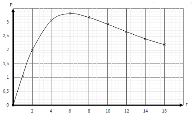
4.2.3.1. Courbe $P=f(r).$
4.2.3.2 Graphiquement $r_{0}=6\;\Omega$ ; on a $r_{0}=r_{\text{max}}$
4.2.4.
$\begin{array}{lrcl}&P&=&\dfrac{U^{2}r}{Z^{2}}\\ \\ \Rightarrow&P_{m}&=&\dfrac{U^{2}r_{0}}{Z^{2}}\quad\text{or }\ \cos\varphi=\dfrac{r_{0}}{Z}\\ \\ \Rightarrow&Z^{2}&=&\dfrac{r_{0}^{2}}{\cos^{2}\varphi} \\ \\ \Rightarrow&P_{m}&=&\dfrac{U^{2}.\cos^{2}\varphi}{r_{0}}\end{array}$
$\begin{array}{rcl}\cos\varphi&=&\sqrt{\dfrac{P_{m}\times r_{0}}{U^{2}}}\\ \\ &=&\sqrt{\dfrac{3.32\;10^{-3}\times 6}{0.2^{2}}}\\ \\ &=&0.7\ \Rightarrow\ \left\lbrace\begin{array}{lcrcr}\varphi&=&\dfrac{\pi}{4}\;rad&=&45^{\circ}\\ \\ \varphi&=&-\dfrac{\pi}{4}\;rad&=&-45^{\circ}\end{array}\right.\end{array}$
Conclusion : $|\varphi|=\dfrac{\pi}{4}\;rad$
4.2.5. L'exception précédente correspond à la résonance d'intensité.
A cet état ; $\varphi=0\ \Rightarrow\ P=UI=\dfrac{U^{2}}{r}$
$U$ étant constante, $P$ est inversement proportionnelle à $r.$
Exercice 5
5.1. .
5.1.1.
$E_{ph(a)}=E_{6}-E_{4}=1.84\;eV$
$E_{ph(b)}=E_{6}-E_{3}=2.82\;eV$
$E_{ph(c)}=E_{3}-E_{1}=2.73\;eV$
5.1.2.
$E_{ph}=\dfrac{hc}{\lambda}\ \Rightarrow\ \lambda=\dfrac{hc}{E_{ph}}$
$\lambda_{a}=\dfrac{6.62\;10^{-34}\times 3\;10^{8}}{1.84\times 1.6\;10^{-19}}=675\;nm$
$\lambda_{b}=\dfrac{6.62\;10^{-34}\times 3\;10^{8}}{2.82\times 1.6\;10^{-19}}=440\;nm$
$\lambda_{c}=\dfrac{6.62\;10^{-34}\times 3\;10^{8}}{2.73\times 1.6\;10^{-19}}=455\;nm$
Elles appartiennent toutes au domaine du visible.
5.2. .
5.2.1. Sources cohérentes : elles présentent un déphasage constant et sont synchrones.
5.2.2.1
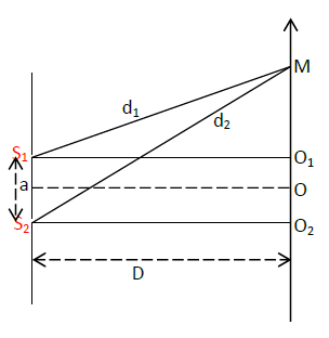
$S_{1}S_{2}=a\ $ et $\ OM=x$
$\Rightarrow\ O_{1}M=x-\dfrac{a}{2}\ $ et $\ O_{2}M=x+\dfrac{a}{2}$ avec $a\prec\prec\prec D$
En considérant les triangles rectangles $(S_{1}O_{1}M)\ $ et $\ (S_{2}O_{2}M)$ on a :
$\begin{array}{lrcl}&d_{1}^{2}&=&D^{2}+\left(x-\dfrac{a}{2}\right)^{2}\ \text{ et }\ d_{2}^{2}\ =\ D^{2}+\left(x+\dfrac{a}{2}\right)^{2} \\ \Leftrightarrow&d_{2}^{2}-d_{1}^{2}&=&2ax\\ \Rightarrow&(d_{2}-d_{1})(d_{2}+d_{1})&=&2ax\end{array}$
On a :
$\begin{array}{lrcl} &\delta&=&d_{2}-d_{1}\quad\text{or }\ a\prec\prec\prec D\\ \Rightarrow&d_{2}+d_{1}&\approx&2D\\ \Rightarrow&d_{2}-d_{1}&=&\delta\ =\ \dfrac{ax}{D}\end{array}$
5.2.2.2 Pour une frange sombre
$\begin{array}{lrcl}&\delta&=&(2k+1)\dfrac{\lambda_{1}}{2}\ =\ \dfrac{a.x}{D}\\ \\ \Rightarrow&x&=&(2k+1)\dfrac{\lambda_{1}D}{2a}\\ \\ \Rightarrow&x&=&\left(k+\dfrac{1}{2}\right)\dfrac{\lambda_{1}D}{a}\end{array}$
5.2.2.3 Pour une frange brillante
$\begin{array}{lrcl}&x&=&k\dfrac{\lambda_{1}D}{2}\quad\text{or }\ d\ =\ x_{5}-x_{3}\\ \\ \Rightarrow&d&=&\dfrac{5\lambda_{1}D}{a}+\left(2+\dfrac{1}{2}\right)\dfrac{\lambda_{1}D}{a}\ =\ \dfrac{15\lambda_{1}D}{2a}\\ \\ \Rightarrow&\lambda_{1}&=&\dfrac{2.a.d}{15.D}\end{array}$
A.N : $\lambda_{1}=\dfrac{2\times 2\;10^{-3}\times 1.024\;10^{-3}}{15\times 486\;10^{-3}}=562\;nm$
5.3. .
5.3.1.
$X_{1}=\dfrac{K_{1}\lambda_{1}D}{a}\quad\text{et}\quad X_{2}=\dfrac{K_{2}\lambda_{2}D}{a}$
Il y a coïncidence pour $X_{1}=X_{2}$
$\begin{array}{lrcl}\Rightarrow&K_{1}\lambda_{1}&=&K_{2}\lambda_{2}\\ \\ \Rightarrow&\dfrac{K_{1}}{K_{2}}&=&\dfrac{\lambda_{2}}{\lambda_{1}}\ =\ 1.5\\ \\ \Rightarrow&\dfrac{K_{1}}{K_{2}}&=&\dfrac{3}{2}\end{array}$
Donc, première coïncidence si $K_{1}=3\;,\ K_{2}=2$
$\begin{array}{lrcl}\Rightarrow&\ell_{1}&=&X_{1}\\ \\ & &=&\dfrac{3\lambda_{1}}{a}\\ \\ & &=&409.7\;10^{-6}\;m\end{array}$
5.3.2. Extinction totale si $X_{1}=X_{2}$
$\begin{array}{lrcl}&(2K_{1}+1)\dfrac{\lambda_{1}D}{2a}&=&(2K_{2}+1)\dfrac{\lambda_{2}D}{2a}\\ \\ \Rightarrow&\dfrac{2K_{1}+1}{2K_{2}+1}&=&\dfrac{\lambda_{2}}{\lambda_{1}}\ =\ \dfrac{3}{2}\\ \\ \Rightarrow&K_{1}&=&\dfrac{3}{2}K_{2}+\dfrac{1}{4}\end{array}$
Si l'une des valeurs $K_{1}\ $ et $\ K_{2}$ est entière, l'autre ne peut pas l'être ; par conséquent on ne peut pas observer une extinction totale sur l'écran.
Ajouter un commentaire